Modeling Instruction: Review of acceleration lab
I’ve been using Modeling Instruction in my physics class for the past five years, and keep wondering how to handle the problem of students who miss the whiteboard sessions (where students share their results and we reach class conclusions). These sessions are critical for student growth, as this is where they are challenged to look for patterns in their data, reflecting on it and comparing it with other groups’ results.
I have created a video PDF file that walks students through the process we would do as a class, which you can find here (PDF format, 3.9 MB). This is an animated PDF file, with voice-over as I write. You can move forward or backward using the navigator buttons, or click on any section of the document to jump to that place in the timeline.
This being my first such attempt at such a video, I would appreciate people’s feedback.
A bit of background on my class graphing methodology
- I don’t ‘linearize’ data (a method where students graph p/t^2 to get a linear relationship).
- I start with hand graphing constant velocity cars, then students use their calculators to conduct a linear regression on the data. They generally like the calculator option because it’s so much faster than hand graphing. (All our students have TI calculators, so we use these instead of Excel–I have a handout that walks them through the process, you can download it here.
- When we graph the data from the accelerating wheel on a ramp, students notice that the relationship is not linear (and they had predicted this from the pre-lab observations). At this point I introduce Quadratic Regression on their calculators, which presents them with y=ax^2+bx+c as the solution. They can determine that “c” is the initial position (plug in t = 0, and y=c), but they do not know what “a” and “b” represent. To solve for that, we move to creating a velocity/time graph:
- Using the “Draw tangent” feature on their calculator, students draw velocities at increasing times (and notice that their velocity values are increasing, again, as they predicted).
- Finally, with a velocity/time graph, we see a linear relationship, and can define the slope as acceleration and the y-intercept as the initial velocity.
- Their final step is to determine what “a” and “b” on the position/time graph equation represent. You’ll have to watch the video to get the answer (or, at least how we decide what you already know–that “a”= 0.5 acceleration and “b” = vi).
- I use “p” for position in my equations and graphs. My students seem to have too big a problem with “x” for position, especially when we plot it on the “y” axis. (When we get to two-dimensional motion, I introduce “x” and “y” as positions.)
Hardware/software
I’m using a Livescribe Echo Smartpen and their Livescribe Desktop to generate the file. The pen allows you to write with normal ink and record all your keystrokes while simultaneously recording your voice. I don’t like that it doesn’t allow different colors, but it’s fairly simple to use, and doesn’t take a lot of post-production work (just save as PDF and the file is created). I also don’t like that it appears to not allow landscape orientation, which would display much nicer on monitors/tablets/etc.
This hardware does not project live, so it’s not something that lends itself to use during class, but it seems to give decent results in just a short amount of time outside of class. This video runs about 15 minutes, and it probably took me 30-45 minutes to create and publish.
There are multiple ways of saving/exporting the final products, and I selected PDF because it is so widely readable, regardless of Mac/Windows/iThing/etc.


